Greenhouse gas (GHG) flux measurements are notoriously noisy. Sensors drift, weather disrupts sampling, and the relationship between soil conditions and gas emissions is non-linear. This post walks through the analytical approach used in environmental GHG research projects, using data from the EucFACE experiment as a reference.
What Are We Measuring?
The primary gases of interest in soil flux studies are:
- CO₂ — produced by microbial respiration and root activity
- CH₄ — consumed or produced by methanotrophic/methanogenic bacteria
- N₂O — produced during nitrification and denitrification
Fluxes are typically measured in µmol m⁻² s⁻¹ (CO₂) or nmol m⁻² s⁻¹ (CH₄, N₂O).
Step 1: Data Ingestion and Quality Control
Raw data arrives as time-series CSV files from automated chambers or manual sampling. The first step is quality control:
import pandas as pd
import numpy as np

df = pd.read_csv("ghg_fluxes_raw.csv", parse_dates=["timestamp"])

# Remove physically implausible values
df = df[df["co2_flux"].between(-50, 50)]
df = df[df["ch4_flux"].between(-500, 500)]

# Flag and remove instrument errors (typically coded as -9999)
df = df.replace(-9999, np.nan)

# Interpolate short gaps (up to 2 consecutive missing values)
df = df.interpolate(method="time", limit=2)
Step 2: Exploratory Analysis
Before modelling, understand the seasonal and diurnal patterns:
import matplotlib.pyplot as plt

df["month"] = df["timestamp"].dt.month
monthly_mean = df.groupby("month")["co2_flux"].mean()

monthly_mean.plot(kind="bar", title="Mean Monthly CO₂ Flux")
plt.ylabel("µmol m⁻² s⁻¹")
plt.tight_layout()
plt.savefig("co2_seasonal.png", dpi=150)
Step 3: Statistical Modelling
For GHG flux data, a mixed-effects model is typically appropriate — it accounts for the repeated-measures structure (multiple observations per chamber per day) and allows for random effects at the site or ring level.
In Python, statsmodels provides mixed linear models:
import statsmodels.formula.api as smf

model = smf.mixedlm(
    "co2_flux ~ temperature + soil_moisture + treatment",
    data=df,
    groups=df["ring_id"]
)
result = model.fit()
print(result.summary())
Key things to check:
- Residual normality (Q-Q plot)
- Homoscedasticity across treatment groups
- Variance explained by the fixed vs. random effects
Step 4: Visualising Results
Interactive dashboards make GHG data accessible to non-specialists. The GHG Estimation Portal was built with Python Streamlit and deployed on Heroku, allowing users to explore modelled flux estimates by site, treatment, and time period without writing any code.
Key charts to include:
- Time series by treatment group (eCO₂ vs. ambient)
- Seasonal cycle overlaid across years
- Scatter plots of flux vs. environmental drivers (temperature, soil moisture)
- Cumulative annual flux estimates with confidence intervals
Summary
| Stage | Key tool |
|---|---|
| Data ingestion & QC | pandas, numpy |
| Exploratory analysis | matplotlib, seaborn |
| Statistical modelling | statsmodels (mixed models), scipy |
| Visualisation & deployment | Streamlit, Heroku |
| Reproducibility | Virtual environments, version-controlled notebooks |
The full modelling workflow for the EucFACE dataset is documented in the GHG Modelling and Geographical Modelling portfolio projects.